Location Estimation - Part 2

In the previous article we attempted to solve this location problem. We used the power of each of a number of signals to roughly estimate our location. We managed to narrow it down to a smallish convex region in the plane shown in green below, which is about 2500 square meters near (-181, 75) . Now we want to go even further and see how accurately we can determine the exact position.

If we take the centroid of this green region as a guess at where we are we then know approximately how far away from each tower we are. We can use this distance along with the speed of sound to work out how long each individual frequency in our received signal is delayed. For example if we are 340.29 meters away from a tower emitting a 3500Hz signal then each sample we received was actually emitted about 1 second earlier so we should phase shift the entire signal 1 second back in time to be using the same time frame as the source.

import math

speed_of_sound = 340.29
centroid_x = -181.666 
centroid_y = -75.373

for tower_x, tower_y in towers:
    dx = centroid_x-tower_x
    dy = centroid_y-tower_y
    distance = math.hypot(dx, dy)
    phase_shift = distance / speed_of_sound
    peaks = find_peaks(times- phase_shift, powers)

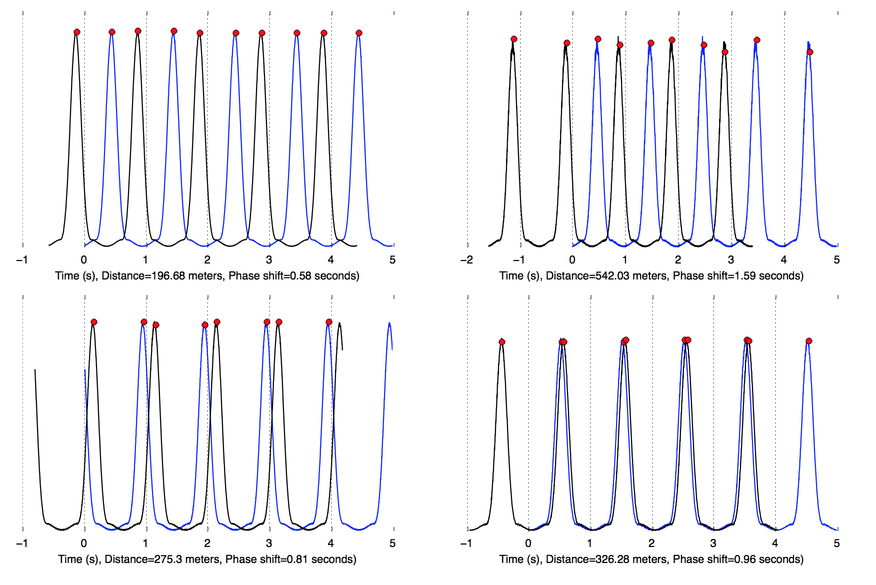
Here is the phase shift of the 350.0Hz tower which is approximately 196.682 meters from our location which means that the source signal is phase shifted -0.578 seconds and moves the time index negative because the tower was emitting a sound before we actually heard anything. The blue peaks shows the 360Hz signal we receive where as the black plot shows the 350Hz signal that was emitted from the source on the same time axis.

Here are a few more towers, the further away the tower the more we have to shift the signal:

All the towers are now on the same time axis but we still don’t know the initial rotation of the towers, nor our exact position. Let’s pick a random initial rotation of the towers and plot what the scene looks like if this were true. What direction would all the towers be pointing in given that we know the phase shift.

This is a disaster. The green dots are the towers and from each tower a number of rays are emitted, there is one ray for each peak of the received signal for that frequency. The rays all go off in different directions unfortunately. Which means that the initial guess at the rotation of the towers was wrong. Let’s try another random rotation:

Looks a bit better but still not obvious. Ideally we want all the rays to intersect at one location this would be the maximum likelihood estimate of the location given the received data. Unfortunately this is not going to happen, because we are dealing with real world data here and there are various sources of noise in this system. For example the rays from a tower don’t go in exactly the same direction because of the imprecision of measuring the times. We have also approximated our initial location which means the phase shift is slightly off. We need a way to quantify how closely the rays all point to the same location. One way to do this is to assume that all the lines should intersect at a specific point and measure the norm of the residuals of the least square solution of this linear system. Here’s an example with three lines:

import numpy as np

points = [
    (-1, -1, 1, 1),
    (1, -1, 0, 1),
    (1, 0, -1, 1)
]
  A = []
  b = []

  for x1, y1, x2, y2 in points:
      m = (y2 - y1) / (x2 - x1) # Check div/0
      c = y1 - (m*x1)
      A.append([-m, 1])
      b.append(c)

  x_sol = np.linalg.lstsq(A, b)[0]
  A = np.array(A)
  b = np.array(b)
  x_est = b - A.dot(x_sol)
  R = np.linalg.norm(x_est)

  print 'Error=', R 

For example if we have three lines that do intersect the norm of the residuals will be zero where as if they don’t the error will increase:

We can use this error value as an objective function and plug our initial guess at the position as well as the range of possible tower orientations -np.pi to np.pi into a BFGS non-linear solver and we should see our unknown position refine to something that agrees with all the towers.

from scipy.optimize import minimize
initial_estimate = [0.0, -181, 75]
result = minimize(objective_func, initial_estimate, method='BFGS')

And away we go:

Awesome. Out pops our most likely position of -179.2, -95.6, which turns out to be within 30 centimeters of the actual location which was at -179.4, -95.3. Not too bad. Here is the data if anyone want to play around with it. It’s interesting to consider the implications of being able to work backwards from a know position and be able to determine the location and power of a missing tower. It’s pretty much the same problem. This is interesting if you’re looking at RADAR. For example the missing Malaysia flight MH370 that was never found last year.

Let’s say there was a someone that could have located the aircraft or at least given an estimate of where it was. By doing so they would also possibly have revealed the capabilities and or locations of their own RADAR systems which might not have been something they wanted. Hopefully this wasn’t the case but it’s something to think about.