The Mighty Kalman Filter

A Kalman Filter is an algorithm for estimating the state of a system from a series of noisy measurements. That’s what I was told, and it confused me. It also doesn’t really do the Kalman filter justice. If we have a bunch of noisy measurements of something why don’t we just take the mean and be done with it? Well the impressive part is estimating the state of a system. This is something that is changing. Let’s says we have a state. This is usually a collection of variables that completely describe where something is and what it’s doing. For example if we are considering a cricket ball hit by a batsman and flying through the air towards the boundary it has a state described by its position which could be three numbers (x, y, z) and its velocity again (vx, vy, vz). In addition the cricket ball is under the effect of gravity so there are forces influencing some of the state. We also assume that the current state can be derived from the previous state. This means that if we know the position and velocity of the ball we can approximately derive the next position of the ball a very small amount of time in the future by integrating forward a little bit. Given these thing the Kalman filter can compute useful thing like the location and velocity of the ball and how sure we are about the estimates.

This sounds a lot more complicated than using a moving average but the Kalman filter cannot be out-performed in certain circumstances. It’s optimal in cases where the model perfectly matches the real system, and noise white and the covariances of the noise are exactly known. These things are seldom true, but it’s impressive how well the Kalman filter does under weaker constraints.

I’ll try a more hand-wavy explanation. The Kalman filter works by alternating between predicting and correcting. It starts with a vague understanding of the state which we can represent by a mean vector (Xk) and covariance matrix (Pk) with the same number of dimensions as there are state variables. It also also has an understanding of the dynamics for the system which are usually state transition and control matrices (A and B). So first it predicts, that is to say it uses its best guess of what the state is and what it understands the dynamics of the system to be to generate the next state using a control vector (Bk) to apply the forces.

Xk = A * Xk + B * Bk

In additions the uncertainty about this new state increases because aren’t doing anything precisely. If we model this - called the process error - by another covariance matrix (Q) we can update our uncertainty like this:

Pk = A * Pk * A.T + Q

So we’ve guessed where we should be, now we correct that guess. We do this by measuring “how far away” our observation (Zk) is from where we think we are and how much we should trust this observation.

Ir = Zk - H*Xp
Ic = H * Pp * H.T + R

So we are working out a term that is used to mix our prediction and the correct. This is called the Kalman gain G which we then use to refine out estimate.

G  = P * H.T * np.linalg.inv(Ic)
Xk = Xp + G * Ir

And we keep doing that over and over. There is a great illustration of the derivation in pictures here. The algebra isn’t too bad, but there are a lot of variables. If we code up these equations we get this little guy:

class KF:
  def __init__(self,A, B, H, Xk, P, Q, R):
    self.A  = A   # State transition
    self.B  = B   # Control
    self.H  = H   # Observation
    self.Xk = Xk  # Initial state
    self.Pk = P   # Initial covariance
    self.Q  = Q   # Estimated error process
    self.R  = R   # Estimated error observations

  def get_state(self):
    return np.array([self.Xk.flat[i] for i in xrange(4)])

  def update(self,Bk,zk):
    Xp = self.A * self.Xk + self.B * Bk
    Pp = self.A * self.Pk * self.A.T + self.Q

    Ir = zk - self.H*Xp
    Ic = self.H * Pp * self.H.T + self.R

    G = Pp * self.H.T * np.linalg.inv(Ic)
    self.Xk = Xp + G * Ir
    size = self.Pk.shape[0]
    self.Pk = (np.eye(size)-G * self.H) * Pp

So how do we use this? We need to model the linear dynamical system too. Let’s go back to the cricket ball flying through the air. We need a way to represent its state, iterate the system and make noisy and un-noisy observations. Here’s a quick and dirty implementation:

class LDS(object):
    def __init__(self):

        angle         = 70
        velocity     = 100
        noise         = 30
        g                = -9.81
        self.noiselevel   = noiselevel
        self.gravity      = np.array([0,g])        
        vx = velocity*np.cos(np.radians(angle))
        vy = velocity*np.sin(np.radians(angle)) 
        self.velocity = [vx, vy]
        self.location     = [0,0] 
        self.acceleration = [0,0]

    def get_location(self):
        return self.location

    def observe_location(self):
        return np.random.normal(self.location, self.noise)

    def observe_velocity(self):
        return np.random.normal(self.velocity, self.noise)

    def integrate(self, dt):
        self.velocity = self.velocity * self.gravity * dt
        self.location = self.location + self.velocity * dt

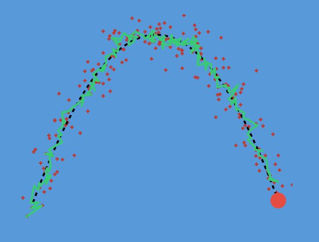
Now we can run our LDS and pump the noisy observations into the KF and plot where we estimate the cricket ball to be. This is what is happening when sports use Hawk-Eye technology. Cameras and RADAR make measurements of where the object (tennis or cricket ball) is and a Kalman filter is used to get more accurate positions and velocities of the object. Before we actually run it, let’s revisit why we don’t just use the average of the noisy estimates, or some kind of moving average. In certain cases, they are the same thing but when the underlying signal is changing the assumption made by a moving average is that the more recent measurements are more important so we lose some information. This can cause havok, if we try to track the location of the cricket ball using a moving average we getting the following:

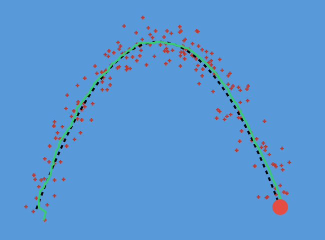
The black dotted line represents the actual trajectory of the ball, the red crosses are the noisy observations and the green is our estimate of the trajectory. Obviously the ball doesn’t do this but the moving average thinks it does. If we drop the Kalman filter:

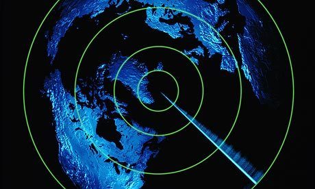
Real nice. We can see that the Kalman filter nicely tracks the position of the cricket ball where we would otherwise have just had the red crosses. Now let’s really put it to the test. In air traffic control you have a RADAR dish measuring where things are approximately. These usually appear as blips on a screen which you see in every action movie ever. You know the one.

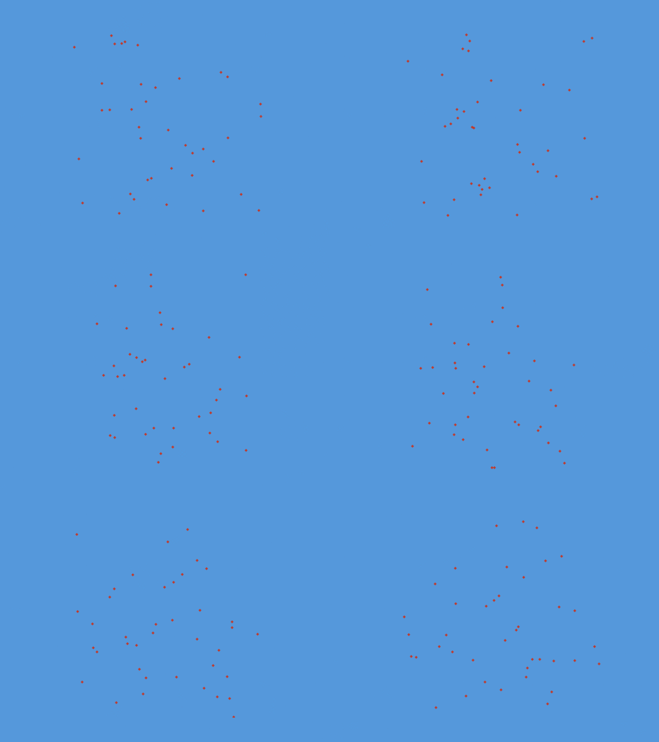
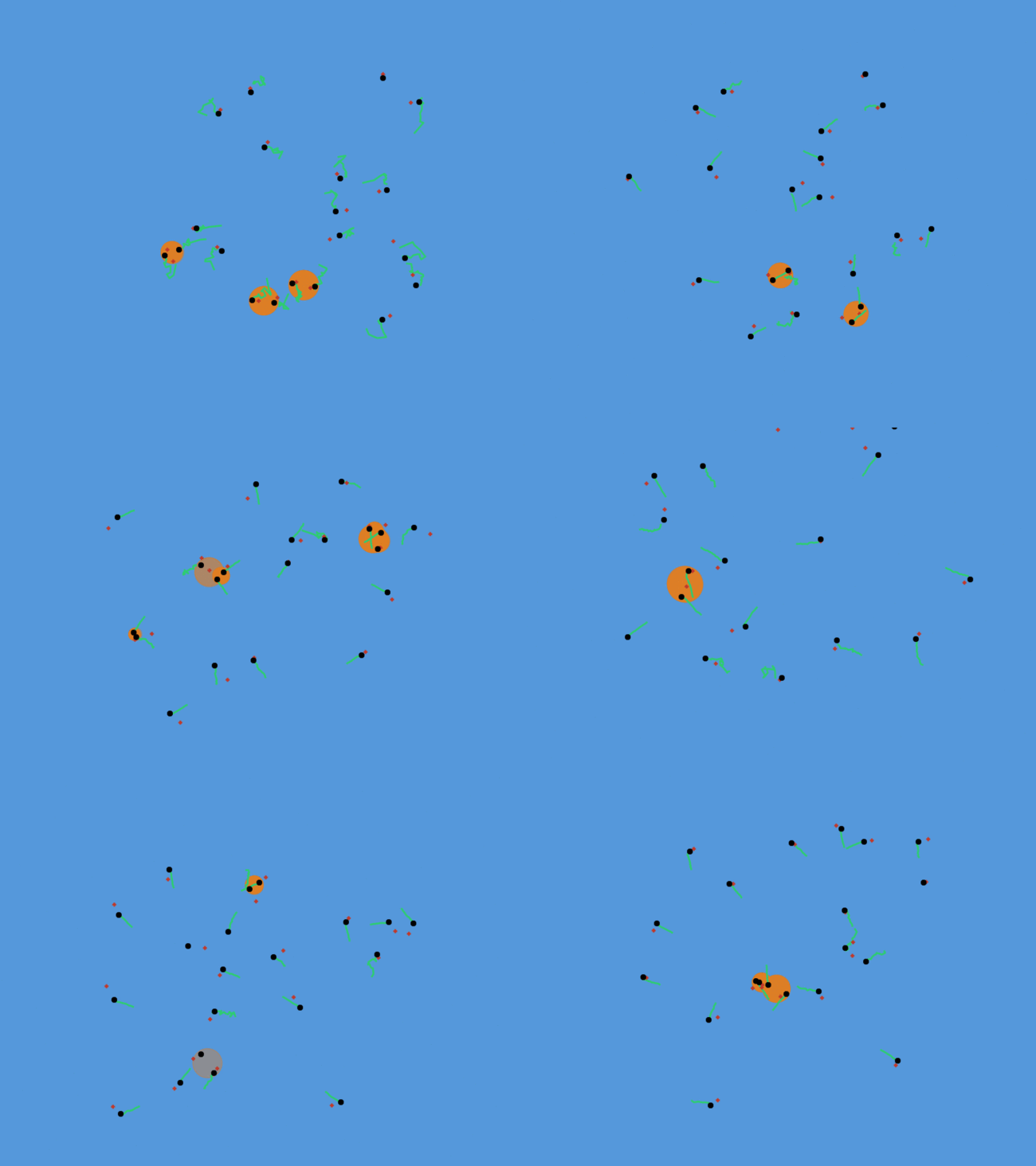
So let’s try and implement a full air traffic control system that is presented with very noisy locations of an unknown number of objects and attempts to concurrently track them and understand when they are in danger of colliding. Firstly here is what things would look like without the Kalman filter. Just a bunch of dots wildly appearing:

Now let say the first time we see a dot appear we assign a Kalman Filter to track it and subsequent dots are part of a same sequence of observations of the same object. When a new dot appears how do we know if it’s another observation of the same object or a new one. The Kalman Filter doesn’t just give us its best estimate of the state but it also given us a measure of its certainty in the form of a covariance matrix (Pk) . So when a new dot appears we can asses how likely that observation is to have come from any of the existing trackers. If it’s outside three standard deviations we assume that it’s a new sequence and assign it its own Kalman filter. If we run this code on the RADAR observations a lot of structure emerges.

Again the red crosses represent the same observations but now we can see estimated locations of the aircraft, how many there are and which direction they are traveling. We can use this information for deconfliction by looking for aircraft within a certain radius of each other (nearby) and with a negative relative velocity (heading towards each-other) and ring them in orange.

So there we have it. Kalman Filters are fast and powerful state estimators that handle noise particularly well. But what if the underlying system is not linear? That’s where the Extended Kalman Filter (EKF) comes in. This is commonly used to fuse IMU data for more accurate GPS readings. The EKF works in a similar way to the Kalman filter while linearizing around the point of interest. This means that we use a first-order approximation of the dynamics which equates to using the Jacobian of the B matrix in place of the state change matrix A. If the dynamics are linear then the Jacobian matrices will all be constant and we get the normal Kalman Filter. I’m not too familiar with the details of the EKF beyond this so maybe this is a topic to re-visit in the future.