Location Estimation - Part 1

We work a lot with GPS data at DroneDeploy. In this article however we are going to look at accurately determining position using sound data instead. This is based on a problem that appeared in the Challenge 24 Programming Competition in 2014. Let’s get started. Let’s say we have a number of towers at different locations. Each tower is emitting a pure tones at a specific frequency and additionally each tower is rotating at 1 Hz. This is what the layout of the towers looks like:

Now let’s say we have a recording of audio received from all these towers and made at a random location. In addition let’s assume that the towers are emitting their tone at approximately (with 20%) the same volume. How do we determine the exact location that the sound was collected? In order to find out where we are, lets first look at the contents of the audio we are receiving. Loading and plotting the spectrogram of the audio with:

def load_wavfile(path):
    fs,samples = scipy.io.wavfile.read(path)
    ts = np.arange(0.0, 1.0 * len(samples) / fs, 1.0 / fs)
    return samples, ts, fs

gives us this diagram:

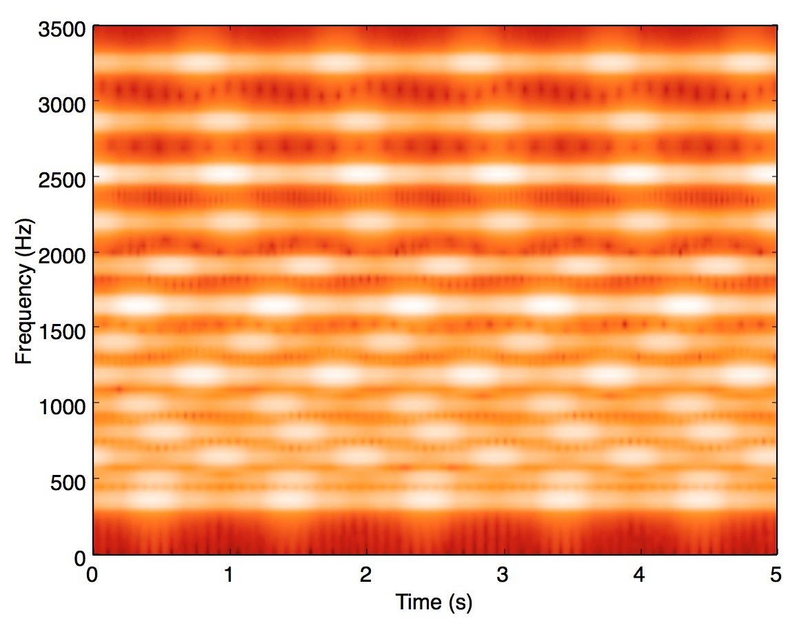
Here we can see the frequencies of each tower are presented and the wiggles in the lines show that the power of the frequency is changing too. This corresponding well with the initial information that the towers are rotating and we’re receiving the largest power value when the tower is point directly towards us. We aren’t going to be considering the rotation of the towers yet - just the peak power of each frequency. The power of the received signal is inversely proportional to the square of the distance from the source. Using this fact we can compute, for any pair of towers which is nearer to out location.

So how do we get the power at each frequency. Normally you could take a FFT of the signal and then measure the power but since we are working with 12 specific frequencies we don’t need a full blown FFT. There is a more efficient way to do this called Geortzel’s algorithm. Goertzel’s algorithm measures the power of a given frequency in a sample. So we slice our original signal into windows. Then convolve the windows with a Hanning window to smooth out the edge effects. Finally we use Goertzel’s algorithm to compute a power series for a given frequency:

def goertzel(samples, freq, sample_rate=44100.0):
    N = len(samples)
    s_prev = 0.0
    s_prev2 = 0.0
    normalizedfreq = freq / sample_rate
    coeff = 2*np.cos(2*np.pi*normalizedfreq)

    for i in xrange(N):
        s = samples[i] + coeff * s_prev - s_prev2
        s_prev2 = s_prev
        s_prev = s

    power = s_prev2*s_prev2+s_prev*s_prev-coeff*s_prev*s_prev2
    return power

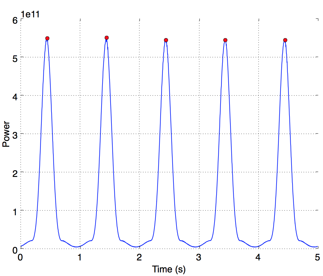
Plotting this data for a single frequency gives us this power series. The power rises and falls as the tower rotates. The next step if picking out the maximum received power at each frequency which is the peak. We can find the peaks but measuring when the power rises above some threshold and then subsequently falls below it. The mid point of these two times is a decent estimate of the peak location. We can then read off the power:

So now we have the maximum power for each tower. If we consider any two towers for example T1 and T2 and the corresponding maximum power we receive from each one P1 and P2, given that we know that these maximums are within 20% of each other at the sources. If P1*0.8 > P2 we are nearer to tower T1 than T2 and vice versa. These actually each represent linear constraints of the form X1 >= A*X2 + B. The points in the plane that are nearer to T1 than T2 is the half-plane whose edge is the perpendicular bisector of the line connecting the two towers. Here’s an illustration where the black line represents the edge of the half plane and the green little points in the direction of the feasible side. T1 and T2 are represented by the blue dots:

So each pair of tower generates a feasible half-plane. We have 12 towers which means we have 12 choose 2 = 66 feasible half-planes. If we take the intersection off all of these half-planes we end up with a convex region which is inside all of them. This is similar to the cutting planes approach used in linear programming and convex optimization tools. Take this intersection gives us this little green area:

This is the set of points in the plane for which the powers of the signals received from all the towers when ordered by magnitude is the same as the ordered distances from this location. In the next post we will try and use this prior information to get an even more accurate location from the same audio file.