Minimum Image Cover
Some applications of photogrammetry require us to collect a number of overlapping aerial images covering an area. The more overlap the better, as more overlap in pairs of images gives us a higher result in some applications. However in other applications we are actually looking for as few images as possible from the set that still cover the area of interest without any gaps.

Framed another way - given a collection of sets, what is the minimum number of those sets that need to be selected such that their union is the union of all of the sets. The sets in our case are defined by taking each location on the ground as a longitude,latitude pair and then finding the set of images that can see that location. We’ll talk about how to enumerate these locations on the ground later. This is called the set cover problem.

Camera Geometry #
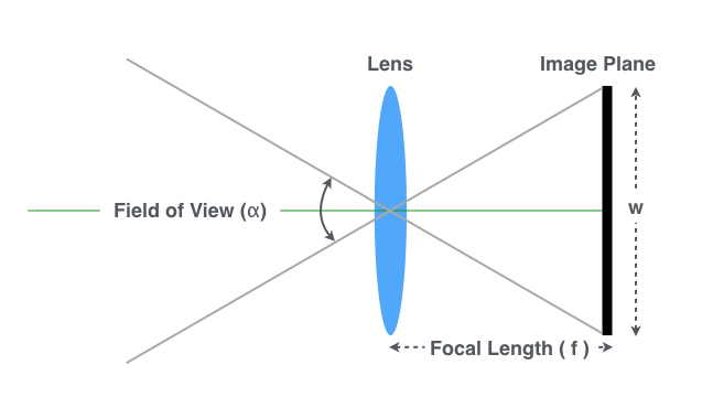
Before we start solving the problem lets generate a dataset of aerial imagery. In order to do that we need to represent an aerial camera at some point in space and the direction in which it is pointing. The location and orientation of the camera together are called the pose and are represented by six values - longitude, latitude, altitude, yaw, pitch and roll. The first three represent position and the last three represent orientation. In addition to this, cameras have a number of intrinsic parameters. For the purposes of our data set we are just going to consider focal length (F) and sensor size. Focal length is the distance over which the camera lens focuses light onto the sensor. The shorter the focal length the wider the field of view. The longer the focal length the smaller the field of view but the higher the ground sampling distance (which is measured in centimeters per pixel). Sensor size is the size of the CCD in the camera, larger sensors (at the same resolution) can represent a larger scene. There are a few different conventions for sensor size and as a result focal length is sometimes given as equivalent focal length as if the sensor were a certain size. In this case we’ll assume that our camera has a 35mm-equivalent focal length of 20mm. Which oddly (by convention) means that the sensor size is 24x36 mm. From these parameters - pose, focal length and sensor size - we can draw this diagram that describes the area on the ground (footprint) that the camera can see which is related to the field of view by the altitude.
This image assumes that the camera is pointing straight down which would generate a clean rectangular footprint (rectangular because the sensor is not square). In reality this is not the case and the aircraft is bumping around and the camera is moving slightly which generates a quadrilateral footprint, also causing some perspective distortion. In order to compute the footprint accurately we can represent the camera with 3 vectors - position, lookat and up. The position vector is the location of the camera in space. The lookat vector is a unit vector in the direction the camera is pointing and the up vector is a unit vector out of the top of the camera to disambiguate the upside down images. We can apply a rotation matrix computed from roll, pitch and yaw to the up and lookat vectors about the camera position to orientate the camera like this.
import numpy as np

def rotate(vector, yaw, pitch, roll):
    Rotz = np.array([
        [np.cos(yaw), np.sin(yaw),  0],
        [-np.sin(yaw), np.cos(yaw), 0],
        [0, 0 ,1]
    ])
    Rotx = np.array([
         [1, 0, 0],
         [0, np.cos(pitch), np.sin(pitch)],
        [0, -np.sin(pitch), np.cos(pitch)]
    ])
    Roty = np.array([
        [np.cos(roll), 0, -np.sin(roll)],
        [0, 1, 0],
        [np.sin(roll), 0, np.cos(roll)]
    ])
    rotation_matrix = np.dot(Rotz, np.dot(Roty, Rotx))
    return np.dot(rotation_matrix, vector)

up = array([0, 1, 0])
position = array([0, 0, 80000]) # 80 meters up
lookat = array([0, 0, -1]) # pointing down
yaw, pitch, roll = 45, 5, 5
up = rotate(up, yaw, pitch, roll)
lookat = rotate(lookat, yaw, pitch, roll)
Now we have a camera pointing in the correct direction we need to compute the four corners of the footprint on the ground. We can do this geometrically by placing the camera sensor plane F-mm away from the camera position in the direction of the lookat and then projecting a ray from the camera position through the four corners of the sensors and into the ground. The point at which the ray intersects the ground - assuming the ground is flat (the ground is not flat) are the four corners of the footprint.
def ground_projection(p, corners):
    k = -position[2] / (corners[2] - position[2])
    return position + (corners-position)*k
Using this code we can generate a bunch of overlapping camera positions covering an area. Here’s a dataset of 100 images taken generated as if a DJI Phantom 4 (F=3.6) was flying over a 250 square meter area at 400m. Now we can return to our set cover problem of finding the minimum number of images that cover the whole area. The whole area in this case is the union of the footprints of the individual images (right). Let’s lay a lattice over the ground to discretize the points of the grounds this is a good approximation of the ground plane and makes the problem easier to solve. (left) We’re now looking for the minimum number of images that cover all the lattice points.

Greedy #
First lets try a greedy approach. Select the image that covers the most uncovered lattice points and add it to your solution set. Continue this until we have covered all the lattice points. This is easy to implement and runs fast, however the result isn’t optimal and we take more images than necessary.
Integer Linear Programming #
Let’s think about the problem another way. Let’s take an example with 6 position on the ground and 5 cameras. Let the 6 positions be variables x1, x2, x3, x4, x5, x6 and the 5 cameras are sets s1 = {x1, x2}, s2 = {x3, x4}, s3 = {x5, s6}, s4 = {x1, x2, x3}, s5 = {x4, x5, x6}.
[x1  x2  x3  x4  x5  x6]
[  s1  ][  s2  ][  s3  ]
[    s4    ][    s5    ]
Let’s assign an inclusion variable i1 .. i6 to each set. We would like to minimize the sum of i1 ... i6 such that for each position on the ground we have included at least one of the cameras containing it. There is one constraint for each element, and also the possibility of duplicate constraints (which can be ignored) if there are two elements that are covered by the same two sets. In this case both x1 and x2 are covered by s1 and s4 hence the first two constraints are the same. Similarly for the last two.
s1 + s4 >= 1
s1 + s4 >= 1
s2 + s4 >= 1
s2 + s5 >= 1
s3 + s5 >= 1
s3 + s5 >= 1
In addition we constrain the variables i1 ... i6 to be {0, 1} we can get an optimal solution to the problem where s1, s2, s3 = 0 and s4, s5=1 which represents the minimum set cover. In reality integer programming itself is dual to Satisfiability which is NP-complete meaning we can’t easily find this solution. But we can use a trick that get us close.
Relaxed Linear Programming #
Let’s relax the condition that i1 ...i6 need to be {0, 1} and let them be floating point numbers between 0 ... 1. Don’t worry too much about the meaning of fractionally including an item in the set this - example with clear that up.
[x1  x2  x3  x4  x5  x6]
[  s1  ][  s2  ][  s3  ]
If we relax the integral constraint the optimal solution 1.5 which is s1, s2, s3 = 0.5. But more importantly if we round up each of these numbers to 1. We still get a solution but possibly lose optimality. In this case we don’t and the rounded solution s1, s2, s3 = 1 is still optimal. However in our previous example
[x1  x2  x3  x4  x5  x6]
[  s1  ][  s2  ][  s3  ]
[    s4    ][    s5    ]
Our rounded solution is 1.5 which rounds up to 3 which is worse than the optimal integral constrained solution of 2 (using just s4 and s5). Our task is now to find a good heuristic way to round up the fractional values. One algorithm to do this is called randomize rounding.
Now we can apply this to our dataset. For each lattice point we compute all the cameras that can see that location and assign that lattice point to a variables. We then set up a linear programming solver to give us a (possibly fractional solution). The code looks like this:
# LP-solver
import pulp

# set up solver
problem = LpProblem("SetCover", LpMinimize)
variables = [ LpVariable("x" + str(var), 0, 1) for var in xrange(100) ]
problem += sum(variables)

# set inclusion constraints
problem += variables[0] >= 1
problem += variables[1] + variables[2] + variables[5] >= 1
...
problem += variables[3] + variables[5] + variables[5] >= 1
problem += variables[1] >= 1

GLPK().solve(problem)

# solution
for v in problem.variables():
    print 'Camera:', v.name, "=", 1 if v.varValue > 0 else 0
Rendering this we see that out of the 100 images we’ve needed to retain only 42 to cover the whole area.
