Fat Albert

I was watching the Fleet Week display by the Blue Angels yesterday and we were talking about if you could determine where an aircraft was based on the sounds you were hearing from the engine.

Say we have an aircraft at some unknown position flying at a constant linear velocity. If the engine is emitting sound at a constant frequency and as soon as we start hearing the engine we start recording the sound. Then given just that audio let’s try and determine how far away the aircraft is and how fast it’s traveling. Here’s a generated sample recording of a source starting 315.914 meters away and traveling at 214 meters per second in an unknown direction.

First let’s make a simplification. We can rotate our frame of reference such that the aircraft is traveling along the x-axis from some unknown starting point. If we look from above the situation looks like this.

When working with audio the first thing to do would probably be to plot the spectrogram and see if we can gleam anything from that. The spectrogram of a WAV file can be plotted using this code:

Fs, audio = scipy.io.wavfile.read('audio.wav')
MAX_FREQUENCY = 2000
pylab.figure(facecolor='white')
pylab.specgram(audio, NFFT = 1024, Fs=Fs, cmap=pylab.cm.gist_heat)
pylab.ylim((100,MAX_FREQUENCY))
pylab.xlim((0,1.1))
pylab.xlabel('Time (s)')
pylab.ylabel('Frequency (Hz)')
pylab.show()

and the result spectrogram which shows the power spectrum of the received signal as a function of time looks like this.

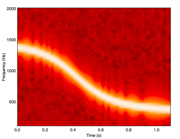
This looks great. Most importantly you can see the Doppler Effect in action because the sound waves are compressing in the direction of the observer. This implies that the aircraft is moving towards us. Other than that there isn’t much that can be gained here. We can look at the inflection point of the spectrogram and infer that this is the point where the aircraft is passing perpendicular to us which corresponds to the actual frequency that the engine is emitting which in this case looks like about 500 Hertz. However we can’t assume that the aircraft will pass us so we probably can’t even take that.

Let’s try something different. Let’s analyze this in the time domain instead. When the aircraft starts emitting sounds at some real time t that sound takes a while before it arrives at the observer. This delay depends on the distance from the observer and the speed of sound. When this first bit of audio arrives at the observer which is t=0 but in “receiver time” the aircraft has already been flying for a while. So this first piece of audio corresponds to a previous location. We don’t know what this delay is because we don’t know how far away the plane way. Since the frequency of the sounds we are receiving are changing because of the Doppler Effect we can’t really rely on frequency analysis either. Let’s instead zoom in and look at the zero-crossings of the signal.

The zero-crossing are the points in time that the signal (regardless of frequency) cross the x-axis. In “real time” there will be a number of times when this happens and they will be constantly spaced by 1/(f*2.0) where f is the frequency of the sounds emitted by the engine. However when we receive the signal and the aircraft is traveling towards us - it will be squashed, and have shorter time between zero-crossings and then further apart as the aircraft flies away. So the signal get’s concertinas in a specific way. Here’s an exaggerated diagram of what is being emitted and what is being received when:

Let’s say the plane is traveling with a speed of v parallel to the x-axis. So its x-coordinates at time t is x0 + v * t (some unknown starting point) and its y-coordinate is R (some unknown distance). Here t is the real time when the signal is emitted. The time for this signal to reach us is:

import numpy as np

def reach_time(x0, v, t, R):
    c = 340.29  # speed of sound
    dt = np.sqrt((x0 + v*t)**2 + R**2)/c
    return dt

The time stamp in received time is just just reach_time(x0, v, t, R) + t - t0 where t0 is the initial and unknown delay for the first signal to reach us. From this we can get the timestamp of the nth zero-crossing knowing that the source frequency is fixed.

import numpy as np

def nth_zero_crossing(n, x0, v, R, f, n0):
    c = 340.29  # speed of sound
    f2 = 2.0*f
    return (np.sqrt((x0 + v*n/f2)**2 + R**2)/c + (n - n0)/f2)

So we’ve got a model that maps the time of a zero-crossing at the source to the time of a zero-crossing in our WAV file. This is a mapping of zero-crossings in the source to zero-crossing in the received signal. Which are the orange lines in this image:

Now we need to extract the zero-crossings from the WAV file so we can compare. We could use some more advanced interpolation but since there are 44100 samples per second in the audio file the impact on the resulting error term should be small. Here’s some code to extract the time of each zero-crossing in an audio file.

import scipy
import numpy as np

Fs, audio = scipy.io.wavfile.read(fn)
audio = np.array(song, dtype='float64')

# normalize
audio = (audio - audio.mean()) / audio.std()

prev = song[0]
ztimes = [ 0 ]

for j in xrange(2, song.shape[0]):
    if (song[j] * prev <= 0 and prev != 0):
        cross = float(j) / Fs
        ztimes.append(cross)
    prev = song[j]

This gives us a generative model where we can select some parameters of the situation and using the nth_zero_crossing compute what the received signal would look like. This puts us in a good position to create an error function between the actual (empirical) data in the audio file and the generated data based on our parameters. Then we can try and find the parameters that minimize this error. Here some code that computes the residue of our generates signal:

import numpy as np

def gen_received_signal(args):
    f2, v, x0, R, n0 = args
    n = np.arange(len(ztimes))
    y = (np.sqrt((x0 + v*n/f2)**2 + R**2)/c + (n - n0)/f2)
    error = np.array(ztimes) - y
    return error

Using a non-linear least squares solver like Levenberg Marquardt we can search for the parameters that best explain our data.

import numpy as np
from scipy.optimize import least_squares

f2 = 1600
v = 100
x0 = -100
R = 10
n0 = 100

args = [f2, v, x0, R, n0]
res = least_squares(gen_received_signal, args)
f2, v, x0, R, n0 = res.x

# compute the initial distance
D = np.sqrt(x0**2+R**2)

print 'Solution distance=', D, 'x0=',x0, 'v=',v, 'f=',f2/2.0

Out of this pops the solution and more. It has also accurately computed the source frequency given some bad initial guesses. Since we aren’t assuming anything about the change in frequency this approach also works when the aircraft does not pass us and is only recorded on approach or flying away from us. In reality the sound would attenuate quadratically over distance but that should not impact this solution because we don’t use amplitudes.